Flood Exposure and Asset Repricing
Flood Risk and Home Values
How FEMA Flood Zone Reclassifications Affect Property Markets
228,002 zip-quarter obs · 2009–2022
by Cameron Keith
Professor Apoorv Gupta · Winter 2026
Econ 66: Topics in Money and Finance
Home values decline gradually after LOMR flood zone reclassification, reaching −2.8% after four or more years. Pre-treatment coefficients near zero confirm the parallel trends assumption.
Research Question
Motivation and contribution
When FEMA updates a flood map through a Letter of Map Revision (LOMR), it officially changes the flood risk classification for properties in the affected area. Properties newly designated as high-risk must carry flood insurance if they have a federally backed mortgage - an immediate, tangible cost. Properties removed from high-risk zones see the opposite: reduced insurance burdens and an implicit signal that flood risk has diminished.
This paper asks a simple question: do housing markets actually capitalize these flood risk signals? If home prices respond to LOMR reclassifications, it suggests buyers and sellers are pricing in government-assessed flood risk. If prices don't respond, it raises questions about whether flood risk information reaches or influences market participants.
Using a staggered difference-in-differences design, this paper exploits variation in the timing of LOMR effective dates across U.S. coastal zip codes from 2009 to 2022 to estimate the effect of flood zone reclassification on home values.
Data & Sample
Sample construction and descriptive statistics
The sample consists of all US coastal zip codes (excluding Alaska, Hawaii, and territories) observed quarterly from 2009 to 2022. Treatment zips are those that received their first (and only) LOMR within the 2009 to 2022 window. ZIP codes with pre-2009 treatment or multiple LOMRs are excluded to ensure clean identification. Control zips consist of never-treated ZIP codes (no LOMR ever) and not-yet-treated ZIP codes (first LOMR after the sample window).
Summary Statistics
| Variable | N | Mean | Std Dev | Min | P25 | Median | P75 | Max |
|---|---|---|---|---|---|---|---|---|
| Panel A: Outcomes | ||||||||
| Home Value Index (Dec 2022 $) | 228,005 | $486,214.62 | $416,676.37 | $32,424.71 | $234,258.39 | $374,152.97 | $594,862.94 | $8,125,586.00 |
| ln(Real ZHVI) | 228,005 | $12.85 | $0.67 | $11.36 | $12.36 | $12.83 | $13.30 | $14.56 |
| ln(NFIP Policies + 1) | 228,005 | 2.46 | 1.80 | 0.00 | 0.98 | 2.08 | 3.71 | 7.87 |
| ln(NFIP Claims + 1) | 228,005 | 0.11 | 0.46 | 0.00 | 0.00 | 0.00 | 0.00 | 8.16 |
| Panel B: Treatment | ||||||||
| Post-LOMR | 228,005 | 0.04 | 0.19 | 0.00 | 0.00 | 0.00 | 0.00 | 1.00 |
| Ever Treated | 228,005 | 0.13 | 0.34 | 0.00 | 0.00 | 0.00 | 0.00 | 1.00 |
| Policy Intensity (per 1,000) | 228,005 | 5.93 | 21.07 | 0.00 | 0.18 | 0.68 | 4.13 | 716.99 |
| Treatment Intensity (per 1,000) | 228,005 | 3.60 | 32.54 | 0.00 | 0.00 | 0.00 | 0.00 | 944.01 |
| Upzoned (into SFHA) | 228,005 | 0.05 | 0.21 | 0.00 | 0.00 | 0.00 | 0.00 | 1.00 |
| Downzoned (out of SFHA) | 228,005 | 0.03 | 0.18 | 0.00 | 0.00 | 0.00 | 0.00 | 1.00 |
| SFHA-Crossing LOMR | 228,005 | 0.08 | 0.27 | 0.00 | 0.00 | 0.00 | 0.00 | 1.00 |
| Panel C: Controls | ||||||||
| NFIP Policies (qtr avg) | 228,005 | 65.21 | 164.11 | 0.00 | 1.67 | 7.00 | 39.67 | 2,624.67 |
| NFIP Avg Premium ($) | 228,005 | $710.36 | $631.82 | $0.00 | $357.67 | $565.67 | $914.10 | $19,570.33 |
| SFHA Zone Share | 228,005 | 0.35 | 0.31 | 0.00 | 0.00 | 0.33 | 0.60 | 1.00 |
| NFIP Claims (qtr avg) | 228,005 | 1.13 | 25.22 | 0.00 | 0.00 | 0.00 | 0.00 | 3,498.00 |
| Zip Population | 228,005 | 19,717.91 | 17,846.46 | 25.00 | 5,236.00 | 15,229.00 | 29,309.00 | 109,931.00 |
| Zip Pop. Density | 228,005 | 4,960.31 | 11,251.76 | 0.90 | 225.60 | 1,571.80 | 4,837.00 | 143,070.70 |
| Panel D: Heterogeneity | ||||||||
| Republican County | 222,846 | 0.50 | 0.50 | 0.00 | 0.00 | 1.00 | 1.00 | 1.00 |
| R Two-Party Vote Share | 222,846 | 0.42 | 0.15 | 0.06 | 0.32 | 0.43 | 0.52 | 0.89 |
| Disclosure: Strict (9 states) | 228,005 | 0.29 | 0.45 | 0.00 | 0.00 | 0.00 | 1.00 | 1.00 |
| Disclosure: Broad (13 states) | 228,005 | 0.61 | 0.49 | 0.00 | 0.00 | 1.00 | 1.00 | 1.00 |
| Estimation sample of U.S. coastal zip codes, quarterly 2009Q1–2022Q4. N = 228,005 zip-quarter obs. | ||||||||
| R Two-Party Vote Share has fewer obs. due to missing election data in some counties. | ||||||||
Pre-Treatment Balance
Comparing pre-LOMR means for treated zips against all-period means for control zips. Significance: * p<0.10, ** p<0.05, *** p<0.01 (Welch t-test).
| Variable | Control | Treated | Difference |
|---|---|---|---|
| Home Value (Dec 2022 $) | $478,848.23 | $474,199.50 | $-4,648.72 |
| Population | 18,542.78 | 21,918.10 | 3,375.32*** |
| Pop. Density (per sq mi) | 5,027.05 | 3,123.25 | -1,903.80*** |
| County Unemp. Rate (\%) | 6.45 | 6.80 | 0.35*** |
| NFIP Policies (qtr avg) | 59.98 | 84.55 | 24.57*** |
| NFIP Avg Premium ($) | $690.42 | $781.76 | $91.35*** |
| SFHA Zone Share | 0.34 | 0.40 | 0.06*** |
| NFIP Claims (qtr avg) | 1.07 | 1.35 | 0.28 |
| Treated: zips with single LOMR during 2009-2022. | |||
| Control: zips with no LOMR. | |||
| Pre-treatment means reported for treated zips. | |||
| Difference = Treated - Control. Welch t-test. | |||
| Significance: *** p<0.01, ** p<0.05, * p<0.1 | |||
Data Sources
External datasets feeding the estimation pipeline
This study integrates 13 external data sources across outcome measurement, treatment construction, controls, heterogeneity analysis, and geographic sample definition. “Scripted” datasets are downloaded automatically via dedicated pipeline scripts; “Manual” datasets require one-time download from their provider. Full pipeline code is on GitHub.
Outcome
| Dataset | Source | Size | Acq. | Pipeline Role |
|---|---|---|---|---|
| Zillow ZHVI (Zip) | Zillow Research Data | ~95 MB | Manual | Primary outcome: monthly home value index by zip code |
| CPI-U (All Urban Consumers) | FRED (BLS via St. Louis Fed) | <1 MB | Scripted | Deflates ZHVI to constant December 2022 dollars |
Treatment
| Dataset | Source | Size | Acq. | Pipeline Role |
|---|---|---|---|---|
| FEMA LOMR Polygons | FEMA NFHL ArcGIS REST API | ~180 MB | Scripted | Treatment events: LOMR effective dates define DiD timing |
| NFIP Policies | OpenFEMA Dataset | ~30 GB | Manual | Policy intensity (treatment scaling), risk direction (upzoned/downzoned) |
| NFIP Claims | OpenFEMA Dataset | ~2.3 GB | Manual | Placebo-like falsification check: a LOMR does not generate flooding, so claims should be unaffected |
Controls
| Dataset | Source | Size | Acq. | Pipeline Role |
|---|---|---|---|---|
| BLS LAUS Unemployment | Bureau of Labor Statistics | ~200 MB | Scripted | County unemployment rate control |
Heterogeneity
| Dataset | Source | Size | Acq. | Pipeline Role |
|---|---|---|---|---|
| Presidential Election Returns | MIT Election Data + Science Lab | ~75 MB | Scripted | Climate skepticism proxy (Republican vote share interaction) |
| State Disclosure Laws | Verified against state statutes | <1 KB | Manual | Asymmetric information mechanism: 9-state disclosure indicator |
Geographic Construction
| Dataset | Source | Size | Acq. | Pipeline Role |
|---|---|---|---|---|
| ZCTA Boundaries (TIGER/Line 2020) | US Census Bureau | ~830 MB | Manual | Zip code polygons for spatial overlay with LOMRs |
| NOAA Coastal Counties | NOAA Office for Coastal Management | ~2 MB | Manual | Defines universe of coastal counties for sample selection |
| Natural Earth Ocean Polygon | Natural Earth Data | ~1 MB | Manual | Removes inland watershed-only counties via spatial join |
| US Zip Code Database | SimpleMaps | ~9 MB | Manual | Zip-to-county crosswalk, population (weights + intensity denominator) |
| State FIPS Crosswalk | US Census Bureau | <1 KB | Manual | State name-to-FIPS mapping for merges across datasets |
Methodology
Identification strategy and econometric specification
This paper uses a staggered difference-in-differences design that exploits variation in the timing of LOMR effective dates across zip codes. The key assumption is that, absent the LOMR, home values in treated and control zips would have followed parallel trends, which is testable in the pre-treatment period.
The event study specification estimates dynamic treatment effects at each year relative to the LOMR:
where z indexes zip codes, t indexes quarters, c(z) maps zip to county, y(t) maps quarter to calendar year, and Ez is the LOMR effective date for treated zip z. The coefficients of interest are the βτ, which trace out the treatment effect at each event-time bin relative to the omitted reference period (τ = −1, the year before the LOMR).
Results
Event study estimates and regression tables
The main event study shows the effect of LOMR flood zone reclassification on log real home values (Real ZHVI, adjusted to December 2022 dollars). Pre-treatment coefficients near zero confirm the parallel trends assumption. Post-treatment, home values decline gradually, reaching −2.8% after four or more years.
ln(Home Values) on LOMR Treatment
| (1) No Controls | (2) Main Controls | (3) Full Controls | |
|---|---|---|---|
| τ = -4 (3+ yrs pre) | -0.0084 | -0.0084 | -0.0084 |
| (0.0076) | (0.0076) | (0.0076) | |
| τ = -3 (2-3 yrs pre) | -0.0002 | -0.0004 | -0.0003 |
| (0.0047) | (0.0047) | (0.0047) | |
| τ = -2 (1-2 yrs pre) | -0.0013 | -0.0014 | -0.0013 |
| (0.0030) | (0.0030) | (0.0030) | |
| τ = 0 (0-1 yr post) | 0.0001 | -4.850e-5 | -2.690e-5 |
| (0.0023) | (0.0023) | (0.0023) | |
| τ = +1 (1-2 yrs post) | -0.0044 | -0.0045 | -0.0046 |
| (0.0040) | (0.0040) | (0.0040) | |
| τ = +2 (2-3 yrs post) | -0.0091 | -0.0093 | -0.0092 |
| (0.0060) | (0.0060) | (0.0060) | |
| τ = +3 (3-4 yrs post) | -0.0139* | -0.0139* | -0.0139* |
| (0.0072) | (0.0071) | (0.0071) | |
| τ = +4 (4+ yrs post) | -0.0285** | -0.0287** | -0.0287** |
| (0.0113) | (0.0113) | (0.0113) | |
| Observations | 228,002 | 228,002 | 228,002 |
| Within R² | 0.0015 | 0.0029 | 0.0030 |
| Zip and county×year fixed effects. Standard errors clustered at county level. Reference period: 12-0 months before LOMR (τ = -1). Already-treated zips (LOMR before 2009) excluded. (1) No controls. (2) Unemployment rate, NFIP policies. (3) Adds avg premium, claims. Significance: *** p<0.01, ** p<0.05, * p<0.1 | |||
Robustness
Diagnostics, parallel trends, and heterogeneity-robust estimation
Parallel Pre-Trends
The identifying assumption requires that treated and control zip codes would have followed parallel home value trajectories absent the LOMR. The raw trends below show treated zips are higher in levels (coastal proximity), but the year-over-year movements track closely. This is consistent with the parallel trends assumption that the zip and county×year fixed effects absorb.
Pre-Period Joint F-Test
A formal joint test of whether all pre-treatment coefficients (τ = −4, −3, −2) are simultaneously zero. Failure to reject supports the parallel trends assumption required for causal identification.
F(3, 338) = 1.04 p = 0.373
Cannot reject the null that all pre-treatment coefficients jointly equal zero. This supports the parallel trends assumption.
Treatment Timing Distribution
The staggered treatment design relies on variation in LOMR effective dates across zip codes. Treatment is spread across the full 2009–2022 window, with increasing frequency in later years as FEMA's mapping modernization program accelerated. This variation identifies the event-time coefficients.
Two-Way Fixed Effects DiD
A simple TWFE DiD with a binary post-treatment indicator estimates the average treatment effect. The coefficient is negative but imprecisely estimated, consistent with the event study showing effects that build gradually over time. A single-period pooled estimate averages early (near-zero) and late (large negative) effects, yielding a small, insignificant average.
| (1) TWFE DiD | |
|---|---|
| Post-LOMR | -0.0070 |
| (0.0080) | |
| County Unemp. Rate (\%) | -0.0022*** |
| (0.0003) | |
| NFIP Policies (qtr avg) | 9.410e-7 |
| (1.010e-5) | |
| Constant | 12.9100*** |
| (0.0022) | |
| Observations | 228002 |
| Within R² | 0.0016 |
| Zip and county×year FE. SE clustered at county level. Significance: *** p<0.01, ** p<0.05, * p<0.1 | |
Unweighted & Geographic Intensity
Unweighted specification: Dropping population weights yields same-direction but smaller and insignificant effects (τ=+4: −0.8% vs −2.8%), consistent with the effect being concentrated in larger, more liquid housing markets where Zillow coverage is strongest.
Geographic intensity: Replacing NFIP policy penetration with the LOMR polygon area / ZCTA area ratio as the intensity measure. Coefficients flip positive and are insignificant, suggesting that raw spatial overlap with reclassified zones is not sufficient; the effect operates through channels tied to insurance exposure and risk information rather than geographic footprint alone.
| (1) (1) | (2) (2) | (3) (3) | |
|---|---|---|---|
| τ = -4 (3+ yrs pre) | -0.0084 | -0.0051 | |
| (0.0076) | (0.0058) | ||
| τ = -3 (2-3 yrs pre) | -0.0004 | -0.0011 | |
| (0.0047) | (0.0036) | ||
| τ = -2 (1-2 yrs pre) | -0.0014 | -0.0016 | |
| (0.0030) | (0.0023) | ||
| τ = 0 (0-1 yr post) | -4.850e-5 | 0.0008 | |
| (0.0023) | (0.0020) | ||
| τ = +1 (1-2 yrs post) | -0.0045 | -0.0006 | |
| (0.0040) | (0.0036) | ||
| τ = +2 (2-3 yrs post) | -0.0093 | -0.0026 | |
| (0.0060) | (0.0052) | ||
| τ = +3 (3-4 yrs post) | -0.0139* | -0.0039 | |
| (0.0071) | (0.0064) | ||
| τ = +4 (4+ yrs post) | -0.0287** | -0.0078 | |
| (0.0113) | (0.0120) | ||
| geo_m4 | -0.0751 | ||
| (0.0461) | |||
| geo_m3 | -0.0201 | ||
| (0.0341) | |||
| geo_m2 | -0.0329 | ||
| (0.0256) | |||
| geo_p0 | 0.0144 | ||
| (0.0209) | |||
| geo_p1 | -0.0002 | ||
| (0.0318) | |||
| geo_p2 | 0.0135 | ||
| (0.0395) | |||
| geo_p3 | 0.0267 | ||
| (0.0520) | |||
| geo_p4 | 0.0536 | ||
| (0.0654) | |||
| Observations | 228,002 | 228,002 | 228,002 |
| Within R² | 0.0029 | 0.0014 | 0.0017 |
| Zip and county×year FE. SE clustered at county level. (1) Main (weighted): baseline specification with population weights. (2) Unweighted: no population weights. (3) Geographic intensity: LOMR area / ZCTA area ratio. Significance: *** p<0.01, ** p<0.05, * p<0.1 | |||
Urban Subsample (Density ≥ 1,000)
Restricting to zip codes with population density ≥ 1,000 per square mile reduces the sample by 44% (228,005 → 127,790 obs; 339 → 155 county clusters) but tests whether the effect concentrates in denser, more liquid housing markets. The binary event study coefficients are uniformly larger in the urban subsample: τ=+4 reaches −3.1% (vs −2.8% in the full sample), and τ=+3 gains a significance star (** vs *). The intensity specification is even sharper: τ=+1 roughly doubles (−1.69*** vs −0.81**) and τ=+2 gains two stars.
Parallel trends still hold (F(3, 154) = 1.72, p = 0.16) but with less margin than the full sample. The pattern is consistent with flood risk capitalization being strongest where housing is most liquid and Zillow coverage is most reliable.
ln(Home Values) on LOMR Treatment (Urban)
ln(Home Values) on LOMR × Policy Intensity (Urban)
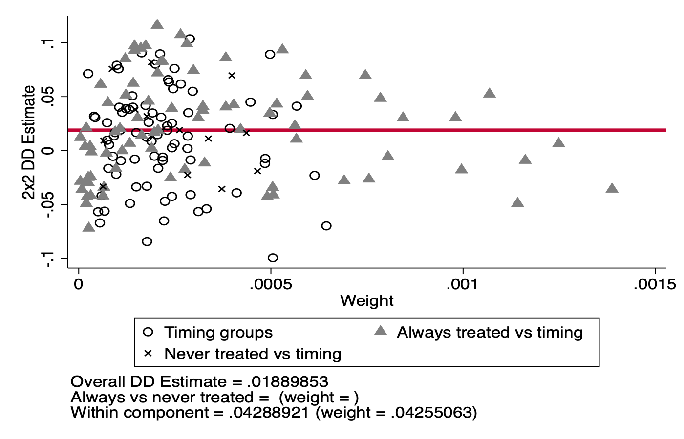
Goodman-Bacon Decomposition
With staggered treatment timing, the TWFE estimator is a weighted average of all 2×2 DiD comparisons, including potentially problematic comparisons that use already-treated units as controls (Goodman-Bacon, 2021). The decomposition below shows the weight and estimate for each comparison type. The Bacon specification uses an annual balanced panel without controls or weights, yielding a positive overall estimate (+0.020) that differs from the main TWFE (−0.007). The event study's intensity specification reveals the heterogeneity that a single DiD number obscures.
Callaway & Sant'Anna Estimator
The heterogeneity-robust Callaway & Sant'Anna (2021) estimator computes group-time average treatment effects separately for each cohort and aggregates them without the problematic comparisons identified by Goodman-Bacon. The ATT estimates are positive (+0.2% to +1.5%), opposite in sign to the main TWFE, and pre-treatment ATTs are significantly positive, suggesting the C&S specification (annual, no controls, balanced panel) does not fully satisfy parallel trends. The discrepancy likely reflects the stripped-down specification required by the csdid package (no continuous controls, no weights, annual collapse).
ln(Home Values) on LOMR (CS Estimator)
Placebo Test: Unemployment as Outcome
Running the main event study specification with county unemployment as the outcome provides a placebo check: if the housing effect is specific to home values, unemployment should be unaffected. However, the pre-treatment interaction test rejects parallel trends (F(3, 338) = 7.22, p = 0.0001), and the τ=+4 bin is significantly negative. This result should be read as a warning sign, not supportive evidence. It implies that the processes generating LOMRs may correlate with local economic changes not fully absorbed by a linear unemployment control. The housing estimates remain the paper's primary results, but readers should note that the placebo does not cleanly rule out macro-level confounds.
Unemployment on LOMR Treatment (Placebo)
Leave-One-Out by State
Each row shows the τ = +4 coefficient when a single state is excluded from the sample. The dashed blue line marks the full-sample estimate. Stability across exclusions indicates that no single state drives the result.
Leave-One-Out by State: τ = +4 Coefficient
Alternative Clustering: County vs State
The baseline specification clusters standard errors at the county level (339 clusters). Clustering at the state level (22 clusters) accounts for broader spatial correlation in shocks, producing wider confidence intervals. The τ=+4 coefficient remains significant under state-level clustering (CI: [−0.055, −0.003]), but τ=+3 loses its borderline significance. Point estimates are unchanged; only the standard errors differ.
ln(Home Values) on LOMR Treatment (Alt. SE)
Limitations
Threats to identification and data quality caveats
Identification & Design
LOMR endogeneity
LOMRs aren’t randomly assigned; FEMA prioritizes areas with recent flood events or development pressure, so reclassification timing may correlate with omitted local shocks.
ZCTA boundary vintage
2020 Census ZCTA boundaries applied to a 2009–2022 panel. Some boundaries shifted between the 2010 and 2020 censuses, potentially misattributing spatial treatment.
County-level clustering
Standard errors clustered at the county level, but treatment varies at the zip level. State-level clustering (shown in Robustness) produces wider confidence intervals.
Data & Proxy Quality
Climate skepticism proxy
Republican vote share is a county-level, coarse proxy for individual climate beliefs.
Disclosure law indicator
Binary, time-invariant, and limited to 9 states. Variation is purely cross-state.
NFIP data quality
reportedCity is 100% unavailable; lat/lng has only 1-decimal precision (~11 km); elevation fields contain sentinel values.
Data
Download research data and replication files
All datasets used in this research are available for download. Data is provided as-is for replication and academic use. The source code for the full data pipeline is available on GitHub.
Replication Package
Everything needed to reproduce all regression results in the paper. Unzip, open Stata, and run do event_study.do.
Individual Files
Event Study Coefficients
Point estimates, standard errors, and 95% confidence intervals for each event-time coefficient across all specifications.
Summary Statistics
Observation counts, means, standard deviations, and percentiles for all regression variables.
Balance Table
Pre-treatment covariate balance between treated and control zip codes with difference tests.
LOMR Treatment Timing
Zip-level treatment data: LOMR dates, number of LOMRs, treatment status, zip characteristics.
Stata Do-File
Complete event study estimation script with all specifications, tables, and figures.
Leave-One-Out State Results
τ = +4 coefficient and 95% CI when each state is excluded from the sample.
Disclosure Law Sources
Statutory citations and verification for the 9 states classified as having mandatory flood zone disclosure during the study period.
Regression Panel
Full zip × quarter panel with ZHVI, treatment indicators, NFIP policies/claims, and BLS unemployment. Generate via the data pipeline on GitHub.
NFIP Policy Panel
Zip × month NFIP policy counts, premiums, claims, and SFHA shares. 997K rows. Generate via the data pipeline on GitHub.
About
Author and acknowledgments
Author
This research was conducted as part of the Economics 66 course. The full paper, data pipeline, and replication code are available on GitHub.
Methodology Note
Data pipeline: Python (pandas, geopandas) for data acquisition, spatial operations, and panel construction. All scripts are reproducible from raw inputs.
Econometrics: Stata (reghdfe) for high-dimensional fixed effects estimation. Callaway & Sant'Anna estimator via the csdid package.
This website: Next.js (static export), D3.js for charts, Tailwind CSS. Deployed on AWS S3 + CloudFront.
Data sources: FEMA NFHL (ArcGIS REST), NFIP policies and claims, Zillow ZHVI, BLS LAUS, Census TIGER/Line, MIT Election Lab, FRED CPI-U, NOAA coastal counties, state flood disclosure laws.